Training and predicting

Data Management's general purpose Machine Learning tools operate in two phases: training and predicting.

In the training phase, the Machine Learning Trainer tool analyzes a set of records containing input features and known results, and attempts to create an optimal model to predict the known results based on the features. The model definition is saved to a file.
In the predicting phase, the Machine Learning Predictor tool loads the model definition created by the Machine Learning Trainer, processes input records containing only features, and predicts the unknown results. The set of features and results used by the Machine Learning Trainer and Machine Learning Predictor must be identical.

Features and results

The Data Management Machine Learning Trainer and Machine Learning Predictor operate on records containing two kinds of data:

Features (also known as inputs or independent variables) are numeric or Boolean values that are input into the Machine Learning process during both training and prediction. In the previous marketing example, the features would be the demographic attributes.
Results (also known as outputs or dependent variables) are numeric or Boolean values that are input into the Machine Learning process during training, and output from the Machine Learning process during prediction. In the previous marketing example, the results would be the RFM scores.

Creating good features

Since the Machine Learning Trainer and Machine Learning Predictor tools require that input data be numeric or Boolean, you may need to preprocess your data to create features of the correct type, tuned to produce the best models. Use the standard Data Management tools such as Calculate to "massage" these kinds of input data into a better form:

Enumerated values like "A", "B", and "C" must be transformed into numbers or Booleans. If the A/B/C values represent actual numbers (such as A=1000, B=2000) you can replace the enumerated values with the corresponding numbers. However, if the enumerated values represent discrete cases (such as A=dog, B=cat, C=llama) you should create a separate Boolean feature for each case (IsDog, IsCat, IsLlama). If you have fewer than 25 cases, the EnumOption parameter on the tool's Fields tab for offers a convenient way to transform such fields.
Missing data: If your input data contains numeric data with Null or Error values (indicating missing data), by default Data Management replaces the Null/Error values with the Mean value. (You can also configure the tool to use the Median or Mode, or report an error.) However, you will usually produce a better model if you "tell" the Machine Learning about the null or error by creating a new feature. For example, if an input feature "Income" may be null, you can create a derived Boolean field which is true for missing or null data by selecting AddMissingDataVariable in the fields grid of the Properties Fields tab.
Text or large enumerated value sets are difficult to map into a useful feature, but there are some cases where you can work with the text. If your text is a large enumerated set of values (for example, State or Province), you may have some success mapping that to a number (the FIPS code of the state) or perhaps creating several derived Boolean features (IsNorthwest, IsMidwest, IsSouth). If the text is arbitrary free-form text, you may find it useful to derive some numeric features (such as word count), or some Boolean features (contains a word from the FirstName lexicon).

Machine learning models

The Machine Learning Trainer and Machine Learning Predictor tools operate with three types of models: regression, classification, and clustering. The regression and classification models perform supervised leaning, meaning that models are trained with known results that are presumed to be correct. The clustering models perform unsupervised learning, meaning that they look for clusters of similar records without knowing any answers in advance.

Regression models

Regression models work with continuous, numeric result values. In the previous marketing example, the RFM scores are continuous result values. Regression models can be used to predict things like "potential sales", "transaction volume", or "credit score." The Data Management repository contains an example of an regression model (see /Samples/MachineLearning):

SinFunction is a synthetic benchmark that has a single input feature named "X" which is in the range (0.0, 3.14159), and predicts a single result, the function sin(X).

Classification models

Classification models are trained on a set of continuous or Boolean features, and a set of discrete Boolean results, exactly one of which is true. The previous marketing example could be recast as a classification problem if, instead of RFM scores, the model addressed a decision such as "send promotional offer?". Other examples of classification problems are:

Fraud detection: "is this a likely fraudulent transaction?"
Creative content selection: is the prospect most likely to respond to the puppy, the race car, or the jewelry image?
Failure prediction: given the current measured conditions (such as temperature, humidity, or vibration) will we experience failure?

Classification models predict the probability that a given result is true, given the feature values. Therefore, the results of a classification model are always floating-point numbers in the range of zero to one. The sum of the probabilities of all results is 1.0 (since only one of them may be true by definition).

Classification models can be trained with a single Boolean result. A "hidden" result is automatically created to represent the "not true" case.

The Data Management repository contains three examples of classification models (see /Samples/MachineLearning):

AnnularRings is a synthetic benchmark classifying points on an (X,Y) grid where X and Y are in the range (-6, +6). Thus, the features are the values of X and Y. The three possible results are a classification of the points based on distance from the origin:
- Class1: Distance from (0,0) is < 2.0
- Class2: Distance from (0,0) is >= 2.0 and < 4.0
- Class3: Distance from (0,0) is >= 4.0
Parity8 is a synthetic benchmark with eight Boolean features. It predicts a single result, the parity of the inputs, which is simply whether the number of features that are True is odd. Note that in this sample, there is a "hidden" classification result corresponding to even.
Titanic predicts passenger survival during the sinking of the RMS Titanic. The feature inputs are variables like age, fare, class, gender, number of siblings, and embarkation point. The single classification result is survived. Note that in this sample, there is a "hidden" classification result corresponding to died.

Clustering models

Clustering models offer a way to discover the underlying structure of your data. They group a set of records together based on a set of features. Clustering groups records by figuring out which data points are closest together, and then determining the centroid, or central point, of each grouping. Clustering methods are based on measuring distances between records and between clusters. Records are assigned to clusters in a way that tends to minimize the distance between records belonging to the same cluster.

The most common use of clustering is segmentation: dividing users, customers, or subscribers into groups of individuals based on similarities that may be relevant to your marketing. While traditional segmentation groups individuals by age, gender, income, and so on, cluster analysis can identify segments using many more dimensions. Using the previous marketing example, one could perform cluster analysis on customer attributes to answer questions like:

What are the demographic characteristics of my best customers?
How do customers behave while purchasing?
What groupings of products do people buy from?

Model fitness

Model fitness is a measure of the expected prediction quality of a model operating on unknown future data. The range of fitness values is [0.0, 1.0], where smaller values are more fit because they represent lower error between actual and expected results. The meaning of the fitness error measurement depends on the model type:

Regression models: fitness is the root-mean-square (RMS) error between the known and predicted results, with result values normalized to the range (0.0, 1.0).
Classification models: fitness is the fraction of incorrectly-predicted results.
Clustering models: if the training data includes defined clusters, an external fitness scoring mechanism is used. Otherwise, internal scoring with the Davies-Bouldin Index is used.

When calculating fitness, Data Management takes steps not to "overtrain" the models. A model so detailed that fits the noise of the training data set rather than its gross statistics is said to be overtrained, and may not generalize well. To avoid overtraining, Data Management takes the following approach:

Subdivide the input training data into training and testing subsets.
Train the candidate models on the training subset.
Measure the fitness of the trained model using a mix of training and testing subsets, usually with emphasis on the testing subset.
Implement various stop conditions to detect when a model starts to overtrain.

The details of this approach may vary depending on the type of model, because some models implicitly incorporate the training/testing division into their overall training process.

Models, optimization, and evolution

The Machine Learning Trainer tool uses an evolutionary algorithm to optimize the models. The first models are randomly created, trained, and tested. The most-fit of these models are retained as the parents of the next generation of models. These parents are mutated into multiple children which are in turn trained and tested. Occasionally, brand-new random models are included to seed solutions that are hard to reach through pure mutation. This process continues until a model is found whose fitness meets your expectations, or until the optimization process has used all its allocated time. You can adjust the parameters of the evolutionary process to control how parents and children are created, mutated, competed, and tested, but the Machine Learning Trainer tool's default settings tend to perform reasonably well.

Machine Learning Trainer

The Machine Learning Trainer processes a vector of features from the input and correlates them with one or more results. It attempts to create a solution or model that can successfully predict future results from features in novel data. It outputs a specification that can be loaded by the Machine Learning Predictor.

While the Machine Learning Trainer has many options for tuning processing, you can usually get good results using the default tool settings.

Configuration parameters

The Machine Learning Trainer has five sets of configuration parameters in addition to the standard execution options:

Optimizer

Output solution file	Name of the file that will contain the solution specification when the training and optimization process is complete.
Parents	Number of solutions selected in each generation for further mutation into children. Default is 10.
Offspring ratio	Number of children derived from each surviving parent during each evolutionary cycle. For example, if Parents=3 and Offspring ratio=8, a total of 3 + 38 = 27 models will be trained and tested each generation. Default is 10.*
Mean mutations	Frequency of mutations performed on child solutions in each iteration of the evolutionary optimizer. Higher numbers will create children that are less like their parents. Default is 1.0.
Adapt mutations	Enables an additional "meta-mutation" strategy that mutates not only the models, but the mutation rate itself, on each generation. This tends to produce better results. Default is On.
Selection strategy	Algorithm used to select the surviving parents in each generation: Elitist: Always choose the parents with the best fitness scores. Default. Tournament: Run a tournament simulation which can increase the diversity of the solutions being searched. Useful in some cases where solutions cannot be found.
Mutation distribution	Selects the distribution of mutation occurrences: Poisson uses Poisson distribution, which tends to produce wilder mutation excursions. Default. Fixed uses uniform distribution, which tends to produce more stable mutation rates.
Maximum generations	Limit on the total number of generations of evolutionary optimization to be performed. Default is 10000.
Total CPU time	Maximum accumulated CPU time to use in the optimization process over all CPU cores on all computers involved in the optimization. Typical values are 30 minutes to 24 hours.
Total wall-clock time	Maximum run time of the optimizer. Typical values are 10 minutes to 10 hours.
Per-model limit Wall-clock time	Maximum run time used to train a single solution. Typical values are 1 minute to 1 hour.
Fitness goal	Desired "fitness" of the solution, expressed as the normalized Root Mean Square error (regression models) or classification error (classification models) between expected results and predicted results. Optimization continues until either the fitness goal is reached or time expires.

Fields

Field	Name of the field.
Usage	Determines how the field is to be used in the model: Input feature: Field contains a numeric or Boolean feature value. Output value: Field contains a numeric or Boolean result value.
Name	Name of the feature or result, if different than Field. Optional.
Enum option	Optionally enumerate the values to create new numeric or Boolean input features. One of: None: Do not enumerate. Non-numeric input data will cause an error. Default. Enum: Enumerate text and non-integer numeric values to create a set of numeric input feature values. Limited to 24 values. Enum w/NoneOfTheAbove: Same as Enum but adds an enumerated value for data not present during the training phase.
Missing data handling	Determines treatment of Null or Error values in features and results. Use the Mean replaces Null/Error values with the mean value. Default. Use the Median replaces Null/Error values with the median value. Use the Mode replaces Null/Error values with the mode value. Skip the Row skips rows containing missing values. Report an error causes training to fail in the presence of Null/Error values.
Add missing data variable	If selected, creates an additional Boolean variable field for the data field, which helps the model learn more efficiently in cases where data is missing. If the data field has a missing value for the row, the value of new variable is set to zero for that row. If there is data present for the row, the value of the new variable is set to one for that row.

Data

Records limit	Sets the maximum number of records used to train the models. You may want to limit the number of records if training times are unacceptable or models are not converging fast enough.
Sampling	Controls how training/testing records are sampled from input records: Nth record: Sample records at a constant interval. Random: Sample records by using a random shuffle.
Auto-normalize inputs	Input features are scanned to determine minimum and maximum values for each column, and linearly mapped onto the range [0.0,1.0]. Default is On.
Auto-normalize outputs	If Mode is Regression, output results are scanned to determine minimum and maximum values for each column, and linearly mapped onto the range [0.0,1.0]. Default is On.
Fitness portion	Defines the fraction of the fitness score that is obtained from the training subset of the data (as opposed to the testing subset). This is normally set to a low number (such as 0.1) to avoid over-training.
Sample	Defines the portion of records that are used for training as opposed to testing. This is normally set to 0.5.

Model Setup

Model type	Type of model to be created: Regression: Used to predict values. Inputs and outputs are continuous values. Multiple outputs are independent of each other. Classification: Used to predict a category. Inputs are a set of continuous or Boolean features, and outputs a set of discrete Boolean results. Clustering: Used to organize data or describe its structure. Partitions input into groups such that items in the same group (or cluster) are more similar to each other than to those in other groups.
Model algorithms	Depending on which Model type is selected, you may select one or more algorithms to be applied by the model: Regression or Classification models: Linear least squares examines the linear relationship between two continuous variables (one input feature and one result output) and finds the best fitting straight line through a set of points. Neural networks pass input features forward through a sequence of layers before turning them into outputs. In each layer, inputs are weighted in various combinations, summed, and passed on to the next layer. Clustering models: Minimum number of clusters and Maximum number of clusters are the minimum and maximum number of clusters to generate. K-means places data points into the specified number of clusters by minimizing the within-cluster sum of squares, clustering numerical data based on Euclidean distance. K-medians places data points into the specified number of clusters by calculating the median for each cluster (rather than the mean used in k-means clustering). K-medoids chooses data points as centers and works with an arbitrary metrics of distances between datapoints, clustering the data set of n objects into k clusters. K-modes is an extension of k-means, using dissimilarities instead of distance, and modes instead of means. It defines clusters based on the number of matching categories between data points, making it useful for clustering categorical variables.
Minimum nodes/layer	If Neural Networks algorithm is selected, the minimum number of nodes allowed in an interior layer. For simple predictive behavior where features tend to have linear influence on results, set Minimum nodes/layer equal to the number of input features / 2. For highly non-linear, interdependent, or "gating" behavior, set Minimum nodes/layer equal to the number of input features.
Maximum nodes/layer	If Neural Networks algorithm is selected, the maximum number of nodes allowed in an interior layer. For simple predictive behavior where features tend to have linear influence on results, set Maximum layers at 2 initially. Once a baseline has been established, test a value of 3 to see if a better model is generated. For highly non-linear, interdependent, or "gating" behavior, set Minimum layers to 3 and Maximum layers to 5. An example of non-linear behavior might be expressed as "propensity to buy increases with income for males, but decreases with income for females."
Minimum layers	If Neural Networks algorithm is selected, the minimum number of layers allowed (this includes the input and output layers, so it must be at least 2).
Maximum layers	If Neural Networks algorithm is selected, the minimum number of layers allowed. This should be greater than or equal to Minimum layers.
Create a "none of the above" output	If model algorithm is Neural networks, selecting this indicates that it is possible for all outputs to be False/0 during training, and creates an additional output variable to represent the False/0 value, if needed.
Cluster measure	If mode is Clustering, the metric used to evaluate cluster quality. The default is Davies-Bouldin index.

Miscellaneous Options

Log to file	If selected, generates log file containing data to help support staff better understand the training process.
Log file name	Path and file to which log will be written.
Log level	Number between 0 (no logging) and 4 (maximal logging).
Output report file	If selected, generates report file containing summary statistics on inputs and output solution.
Report file name	Path and file to which report will be written.
Use fixed seed	If selected, forces the random-number generator used internally by the Trainer to start at the same value. Useful for debugging.

Configure the Machine Learning Trainer

Select the Machine Learning Trainer tool, and then go to the Optimizer tab on the Properties pane.
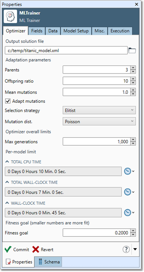
- Select Output solution file and specify the file in which the optimized model will be saved when the training and optimization process is complete.
- Adaptation parameters control the overall behavior of the optimizer. Unless you are familiar with the Machine Learning Trainer tool, we recommend leaving these at the default settings. See Models, optimization, and evolution and Configuration parameters for details.
- Optimizer overall limits and Per-model limit define stop points for the optimization process. When optimization stops, the best model found to that point is saved as the solution.
- Select Max generations to adjust the number of generations to be explored.
- Specify Total CPU time to limit the aggregate CPU time consumed by all threads.
- Specify Total wall-clock time to limit time elapsed from the start of optimization.
- Specify Per model - Wall-clock time to limit models with iterative training processes (such as neural networks) to time elapsed from start of optimization. Not all models will honor this limit.
- Specify a Fitness goal that reflects the quality of the training data. Guidelines:
  - Synthetic benchmarks: 0.01
  - Typical real-world data: 0.1
  - Noisy real-word data: 0.2
You can also set a fitness goal of zero and let the clock run out, then evaluate the quality of the solution.
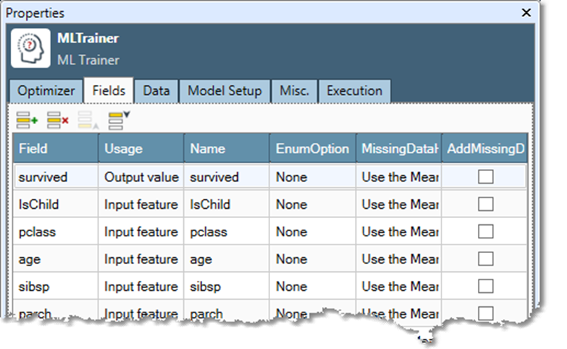
Select the Fields tab and map input fields to features and results. See Creating good features for more information.
For each feature or independent variable:
- Choose the field in the Field column.
- Select Input feature in the Usage column.
- Optionally, specify a different feature name in the Name column.
For each result or dependent variable:
- Choose the field in the Field column.
- Select Output value in the Usage column
- Optionally, specify a different result name in the Name column.
- Select an EnumOption to enumerate the values to create new Boolean features, or accept the default choice of None.
- Select a MissingDataHandling option, or accept the default choice to Use the Mean.
- Optionally, select AddMissingDataVariable to create a Boolean field which is true for missing or null data.
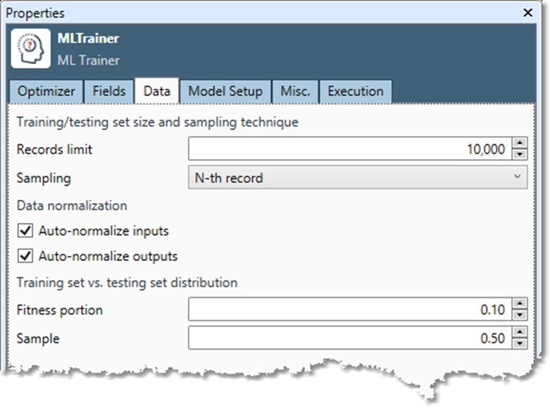
Select the Data tab to adjust model fitness options:
- Records limit sets the maximum number of records used to train the models. If training times are unacceptable or models are not converging fast enough, set a lower limit.
- Sampling defines how training/testing records are sampled from input records:
- Nth record samples records at a defined interval.
- Random samples records using a random shuffle.
- Auto-normalize inputs should be selected unless your input features have been normalized to the range (0.0, 1.0).
- Auto-normalize outputs should be selected unless your output results have been normalized to the range (0.1, 0.9) or Mode is Classification.
- Fitness portion should be set to a low number such as 0.1 to avoid over-training.
- Sample is normally set to 0.5.
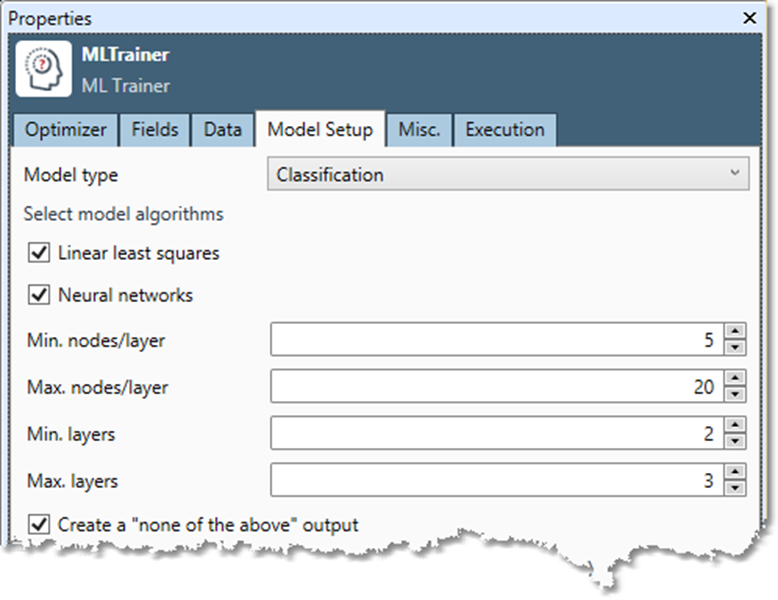
Select the Model Setup tab to define the "universe" of models that can be considered for a solution.
- Select Model type and select the type of model to be created: Regression, Classification, or Cluster.
- Select one or more model algorithms, and then configure options.
Select the Misc tab to define logging and reporting or enable a random-number generated "fixed seed."
Optionally, go to the Execution tab, and then set Web service options.

Machine Learning Predictor

The Machine Learning Predictor loads the predictive models generated by the Machine Learning Trainer and executes them on input features to produce results.

Configuration parameters

The Machine Learning Predictor has two sets of configuration parameters in addition to the standard execution options:

Configuration

Solution file

Name of the file containing the model generated by the Machine Learning Trainer.

Fields

Input mapping: Model Input (feature)	Maps model feature field (as configured in the Machine Learning Trainer that generated the solution) to numeric or Boolean input field.
Result mapping: Model Output (prediction)	Maps result field (as configured in the Machine Learning Trainer that generated the solution) to numeric or Boolean output. Field is optional but must be a float.

If you specify a Solution file that was generated by an older version of Data Management, the Model Input (feature) and Model Output (prediction) lists may not display any parameters to be mapped. If this is the case, re-run the Machine Learning Trainer project to generate an updated solution file.

Configure the Machine Learning Predictor

Select the Machine Learning Predictor tool, and then go to the Configuration tab.
Specify a Solution file previously generated by the Machine Learning Trainer.
Select the Fields tab and map input and result fields to features and results.
- In the Input mapping grid, map each Model Input (feature) or independent variable to the corresponding field in the Field column.
- In the Result mapping grid, map each Model Output (prediction) or dependent variable to the corresponding field in the Field column.

If the solution file you specified in Step 2 was generated by an older version of Data Management, the Model Input (feature) and Model Output (prediction) lists may not display any parameters to be mapped. You must re-run the Machine Learning Trainer project to generate an updated solution file.

Optionally, go to the Execution tab, and then set Web service options.